Examples

A worked, end-to-end run on the bundled policy-sentiment task: get the data, run a model, read the row-level output, score it against the human labels, and compare multiple configurations. Everything here works against the task shipped with the package, so you can follow along before plugging in your own data.

The policy-sentiment task

policy-sentiment asks four questions about short political texts, one of each annotation type:

Field	Type	Values
Policy Sentiment_Explicit evaluation	checkbox	1 / 0
Policy Sentiment_Direction	dropdown	positive · negative · mixed · no clear sentiment
Policy Sentiment_Intensity	Likert	1–5
Policy Sentiment_Evidence	textbox	short free text

The ground-truth.csv holds the human labels in those columns, plus metadata (doc_id, title, topic, speaker_type) and the text to annotate.

1. Get the task

Copy the bundled task into a local folder you control:

from codebook_lab import copy_example_task

copy_example_task("policy-sentiment", "tasks")

This writes tasks/policy-sentiment/codebook.json and tasks/policy-sentiment/ground-truth.csv.

2. Run one experiment

from codebook_lab import ExperimentSpec, run_experiment

result = run_experiment(
    ExperimentSpec(
        task="policy-sentiment",
        model="gemma3:270m",
        use_examples=False,
        prompt_type="standard",
        process_textbox=True,
        country_iso_code="IRL",
    ),
    task_root="tasks",
)

print(result.experiment_directory)
print(result.metrics.summary_text)

Lab strips the human label columns before prompting, runs the model on each row, writes the outputs to a timestamped directory, and scores the predictions against the held-out labels.

3. Inspect the row-level output

output.csv keeps the metadata and text, with the model’s predictions in the same annotation columns (illustrative):

doc_id	Policy Sentiment_Explicit evaluation	Policy Sentiment_Direction	Policy Sentiment_Intensity	Policy Sentiment_Evidence
ps_001	1	positive	5	“sensible compromise”
ps_002	1	negative	2	“financing assumptions are unrealistic”
ps_003	0	no clear sentiment	3	“”

Because the columns match the codebook, you can merge output.csv back against ground-truth.csv on doc_id to inspect individual disagreements.

4. Read the metrics

result.metrics.summary_text prints a quick overview, and the full results land in the tidy metrics tables under outputs/metrics/ (illustrative):

outputs/metrics/policy-sentiment_metrics_log.csv

run_id	column	metric	value
run_a1b2	Policy Sentiment_Direction	f1_macro	0.71
run_a1b2	Policy Sentiment_Direction	percentage_agreement	0.80
run_a1b2	Policy Sentiment_Intensity	quadratic_kappa	0.66
run_a1b2	Policy Sentiment_Evidence	norm_levenshtein	0.52

The companion policy-sentiment_metrics_log_runs.csv carries one row per run with the model, prompt, and sampling configuration alongside runtime, character counts, energy, and emissions — joined back to the metrics via run_id. See Outputs & Metrics for the full field list and guidance on choosing metrics.

5. Compare configurations

The point of CodeBook Lab is comparison. Because the codebook and labels stay fixed, you can isolate one variable at a time – here, model choice and zero-shot versus few-shot prompting.

This example runs the full 20-row bundled task with two recent 4B local models: qwen3:4b and gemma3:4b. It disables textbox generation so the benchmark focuses on the checkbox, dropdown, and Likert fields while still using the real metrics and efficiency pipeline. The code below assumes the models are already available locally in Ollama. If needed, run ollama pull qwen3:4b and ollama pull gemma3:4b first.

from codebook_lab import ExperimentSpec, copy_example_task, run_experiment

copy_example_task("policy-sentiment", "tasks")

specs = [
    ExperimentSpec(
        task="policy-sentiment",
        model="qwen3:4b",
        use_examples=False,
        reasoning=False,
        process_textbox=False,
        country_iso_code="IRL",
    ),
    ExperimentSpec(
        task="policy-sentiment",
        model="qwen3:4b",
        use_examples=True,
        reasoning=False,
        process_textbox=False,
        country_iso_code="IRL",
    ),
    ExperimentSpec(
        task="policy-sentiment",
        model="gemma3:4b",
        use_examples=False,
        process_textbox=False,
        country_iso_code="IRL",
    ),
    ExperimentSpec(
        task="policy-sentiment",
        model="gemma3:4b",
        use_examples=True,
        process_textbox=False,
        country_iso_code="IRL",
    ),
]

for spec in specs:
    run_experiment(
        spec,
        task_root="tasks",
        output_root="outputs",
        pull_model=False,
    )

Each run appends to the same two linked metrics tables:

import pandas as pd

metrics = pd.read_csv("outputs/metrics/policy-sentiment_metrics_log.csv")
runs = pd.read_csv("outputs/metrics/policy-sentiment_metrics_log_runs.csv")

joined = metrics.merge(runs, on="run_id")

field_f1 = joined[
    (
        joined["column"].isin(
            [
                "Policy Sentiment_Explicit evaluation",
                "Policy Sentiment_Direction",
                "Policy Sentiment_Intensity",
            ]
        )
    )
    & (joined["metric"] == "f1")
]

efficiency = runs[
    [
        "run_id",
        "model_id",
        "use_examples",
        "n_queries",
        "avg_inference_time_per_query_s",
        "avg_output_chars_per_query",
        "avg_energy_kwh_per_query",
    ]
]

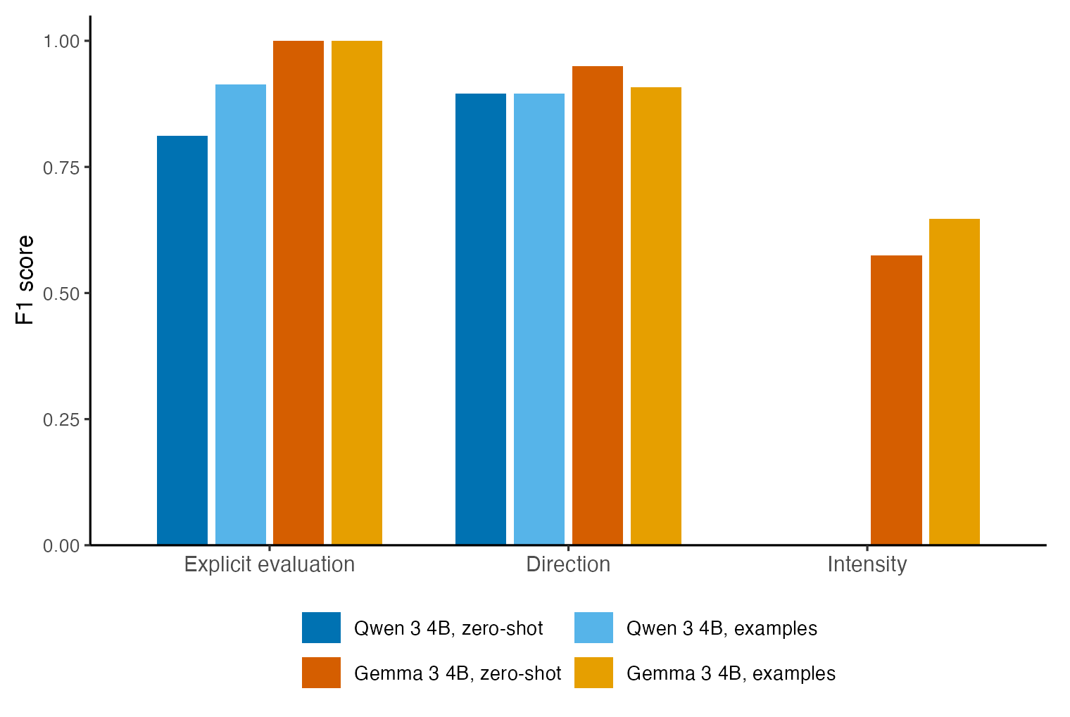
These are real figures from the full benchmark, run locally with Ollama on an Apple M2. Your exact numbers will vary by machine, model build, and model response validity. The plots are produced from the joined tables with ggplot2 and theme_classic().

Run	Explicit evaluation F1	Direction F1	Intensity F1
Qwen 3 4B, zero-shot	0.812	0.896	0.000
Qwen 3 4B, examples	0.913	0.896	0.000
Gemma 3 4B, zero-shot	1.000	0.949	0.575
Gemma 3 4B, examples	1.000	0.908	0.647

Field-level F1 scores for four policy-sentiment benchmark runs.

Run	Avg seconds/query	Avg output chars/query	Avg energy/query (kWh)
Qwen 3 4B, zero-shot	2.52	110	0.00000777
Qwen 3 4B, examples	3.00	71	0.00000620
Gemma 3 4B, zero-shot	2.06	19	0.00000373
Gemma 3 4B, examples	2.62	20	0.00000500

Efficiency measures for the same four policy-sentiment benchmark runs.

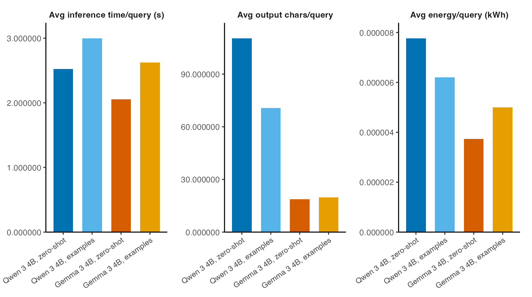
The tradeoff is visible: qwen3:4b scores well on explicit evaluation and direction, but in this run it did not return valid Likert values for intensity, which triggered retries and raised the query count to 80. gemma3:4b completed the same task in 60 model calls and handled all three scored fields. Adding examples improved Qwen’s explicit-evaluation F1 and Gemma’s intensity F1, but it also increased average inference time and prompt size.

The CSVs used for the tables and plots are included with these docs:

• Field-level F1 metrics
• Run configuration and efficiency metrics

The important pattern is the same for larger benchmarks: join on run_id, pick the field and metric you care about, then compare those values against the run configuration and efficiency columns.

Next steps

• Tasks — the codebook.json / ground-truth.csv format for your own data.
• Annotation Types — checkbox, dropdown, Likert, textbox, and span fields.
• Experiments — single runs, sweeps, custom prompt wrappers, and running without ground truth.
• CodeBook Studio — designing a codebook and annotating in the browser.